Fall 2025 • Machine Learning Course
Kernel SVMs from Scratch
Support vector machines are one of the most important classical classifiers, and kernels are what let a linear method learn curved decision boundaries without ever computing the curved features directly. Calling a library hides all of that. In this assignment we built binary SVM classifiers from scratch in NumPy, writing every objective, constraint matrix, and kernel by hand. CVXOPT was used only as the quadratic program solver and SciPy only for unconstrained minimization, with no scikit-learn anywhere.
What We Built
- Primal form. A linear classifier with L2 regularization, trained two ways: the hinge loss written as a quadratic program for CVXOPT, and the smooth ExpLinear loss minimized directly with SciPy.
- Adjoint form. The same two losses rewritten in terms of the training points, so any kernel can be plugged in: linear, polynomial of degree 2 and 3, and Gaussian of several widths.
- Dual form. The classic SVM dual with the hinge loss, solved as a quadratic program over the kernel matrix, with its own classifier for new points.
- Model selection. 5 fold cross validation over the regularization strength λ and seven kernels, run on handwritten 4s and 9s from MNIST.
The synthetic tests used three datasets of increasing difficulty: Model 1 is linearly separable, Model 2 needs an oval boundary, and Model 3 is two interleaving moons.
Results
Test accuracy by kernel (adjoint form)
| Kernel | ExpLinear M1 | ExpLinear M2 | ExpLinear M3 | Hinge M1 | Hinge M2 | Hinge M3 |
|---|---|---|---|---|---|---|
| Linear | 0.9889 | 0.5695 | 0.8840 | 0.9863 | 0.6034 | 0.8802 |
| Poly (d = 2) | 0.9859 | 0.9795 | 0.8826 | 0.9831 | 0.9713 | 0.8793 |
| Poly (d = 3) | 0.9751 | 0.9638 | 0.9929 | 0.9699 | 0.9600 | 0.9862 |
| Gauss (σ = 1) | 0.9723 | 0.9672 | 0.9977 | 0.9637 | 0.9657 | 0.9946 |
| Gauss (σ = 0.5) | 0.9587 | 0.9625 | 0.9982 | 0.9596 | 0.9588 | 0.9981 |
A linear boundary is close to guessing on the oval dataset (57% to 60%), while polynomial and Gaussian kernels lift it to about 96% to 98%.
Best kernel and loss for each dataset
| Dataset | Best kernel | Best loss | Test accuracy |
|---|---|---|---|
| Model 1 (linear) | Linear | ExpLinear | 0.989 |
| Model 2 (oval) | Poly (d = 2) | ExpLinear | 0.979 |
| Model 3 (moons) | Gauss (σ = 0.5) | Hinge | 0.998 |
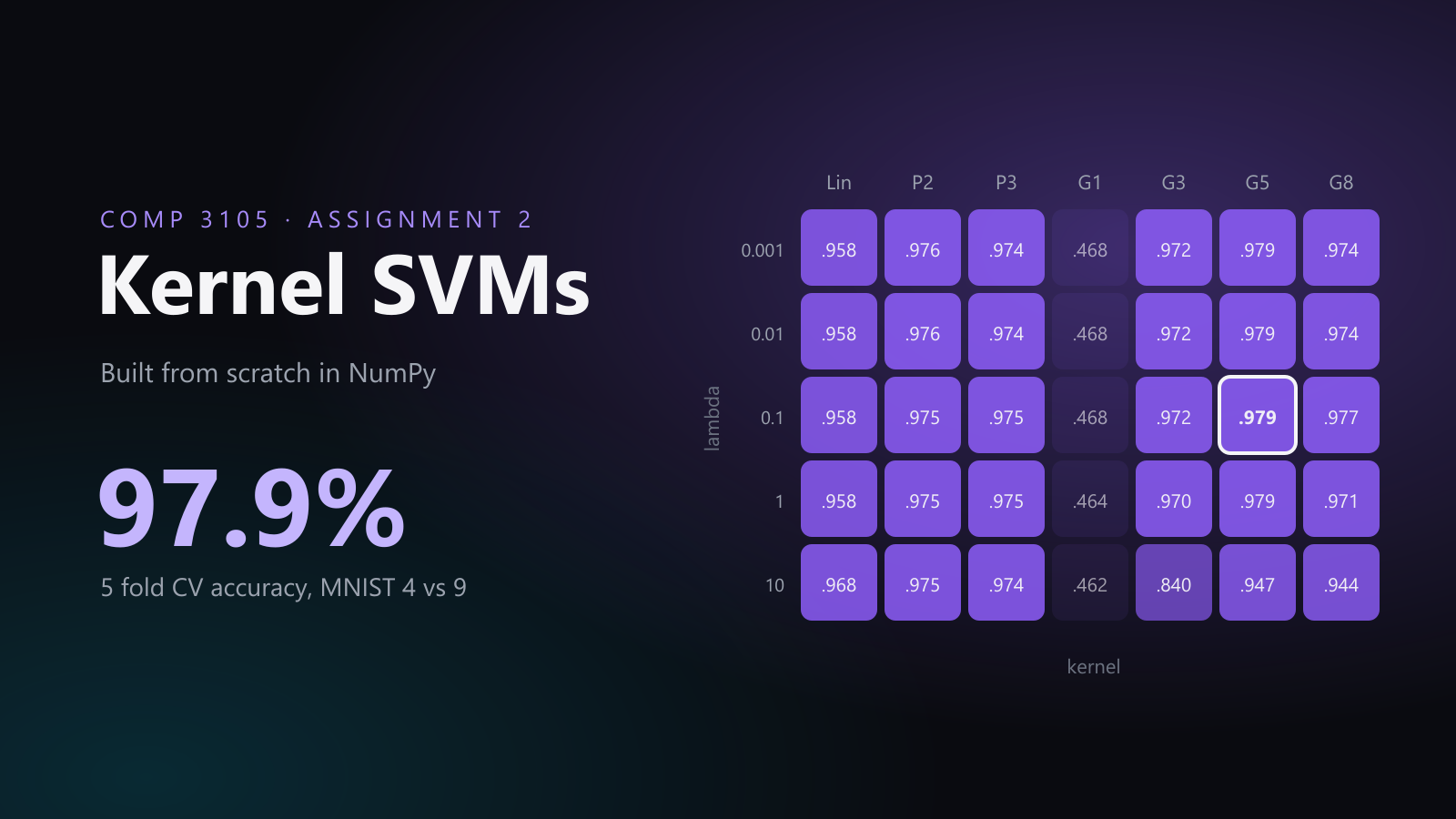
MNIST 4 vs 9: 5 fold cross validated accuracy (dual form)
| λ | Linear | Poly 2 | Poly 3 | Gauss 1 | Gauss 3 | Gauss 5 | Gauss 8 |
|---|---|---|---|---|---|---|---|
| 0.001 | 0.958 | 0.976 | 0.974 | 0.468 | 0.972 | 0.979 | 0.974 |
| 0.01 | 0.958 | 0.976 | 0.974 | 0.468 | 0.972 | 0.979 | 0.974 |
| 0.1 | 0.958 | 0.975 | 0.975 | 0.468 | 0.972 | 0.979 | 0.977 |
| 1 | 0.958 | 0.975 | 0.975 | 0.464 | 0.970 | 0.979 | 0.971 |
| 10 | 0.968 | 0.975 | 0.974 | 0.462 | 0.840 | 0.947 | 0.944 |
We chose a Gaussian kernel with σ = 5 and λ = 0.1: it ties for the best accuracy, 97.9%, while keeping enough regularization to avoid overfitting to unusual samples.
What We Learned
- The kernel matters far more than the loss: ExpLinear and hinge stayed within about 3 points of each other everywhere, while switching kernels moved accuracy by as much as 41 points.
- Match the kernel to the data. The linear kernel won on linearly separable data, and Gaussian kernels won on the moons, reaching 99.8% test accuracy.
- Flexible kernels overfit. A narrow Gaussian (σ = 0.5) hit 100% training accuracy on every dataset but lost up to 4.1 points on the test set.
- On clean data, more regularization is not free: raising λ slightly lowered accuracy, because there was little noise to protect against.
Completed as a pair assignment with a teammate. The code stays private since it is graded coursework.
 Python
 NumPy
 pandas