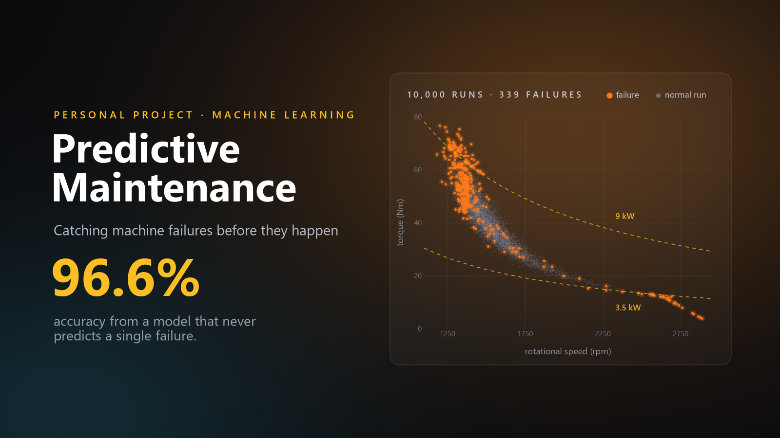
Mini Research • Predicting Machine Failures
Predictive Maintenance
Every machine wears out, no matter how well it is built. Its quality decides how well it performs and how long it lasts, but sooner or later, something gives.
To avoid breakdowns in the middle of production, many factories replace parts on a fixed calendar, whether the part needs it or not. It works, but it is wasteful: the U.S. Department of Energy lists “unneeded maintenance” as a built in cost of calendar based programs [2], and Siemens points to lines closed for no reason and expensive spare parts kept on the shelf just in case [1]. Wait too long instead, and a single hour of unplanned downtime in a large car plant now costs about $2.3 million [1].
This project asks a simple question:
Can a machine's own sensor readings warn us before it fails?
We dig into what a machine reports about itself (temperature, speed, torque, and tool wear) and test whether machine learning can turn those readings into an early warning. The hard part is that failures are rare, about 3 in every 100 runs. A model that always says “everything is fine” would be right 96.6% of the time and still miss every single breakdown.
So instead of just training a model, we ran it like a small research study: explore the data, form hypotheses, test them with models chosen for a reason, and dig into the failures the final model still misses. The result catches more than twice as many failures as a simple baseline, and about two in three of its alerts are real.
10,000
machine runs, 6 input features
3.39%
of runs end in a failure
5
models compared with 5 fold cross validation
69%
of the final model's alerts were real failures
How This Helps in a Real Factory
Unplanned downtime is one of the most expensive problems in manufacturing. Siemens' 2024 survey of industrial companies puts numbers on it [1]:
−$1.4T
lost every year by the world's 500 largest companies, 11% of their revenue
−$2.3M
the cost of one hour of downtime in a large car plant
27 h
of unplanned downtime per month at an average large plant
−$253M
yearly cost of downtime for an average large plant
Predictive maintenance is how plants fight back. In independent surveys gathered by the U.S. Department of Energy, plants that started a working predictive maintenance program reported these average results [2]:
25 to 30%
lower maintenance costs
70 to 75%
fewer breakdowns
35 to 45%
less downtime
+10x
return on the investment
In hours: an average large plant loses 27 hours a month to unplanned downtime [1]. Cutting that by 35 to 45% [2] gives back about 9 to 12 hours of production every month, more than a full 8 hour shift.
Here is what our analysis adds to that picture:
- Less time checking healthy machines. Instead of inspecting everything on a calendar, the crew checks only what the model flags: 52 of our 2,000 test runs, about 2.6%, and two in three of those were real failures.
- Fewer surprise breakdowns. The model caught 36 of 68 failures before they happened, more than twice the 16 caught by a simple baseline.
- A dial, not a fixed answer. The decision threshold trades caught failures against false alarms. A plant where a breakdown costs far more than an inspection can lower it and catch more failures (Table 7).
- Operating rules a technician can read. Risk concentrates in a few zones: the highest fifth of torque fails at 11.5%, the lowest fifth of rotational speed at 12.2%, and tool wear above about 174 minutes at 8.1%, against 3.4% overall.
- Known blind spots. The error analysis shows which failures the model tends to miss, so those cases can be covered by inspections instead of trusting the model.
What a plant cares about is not accuracy but the alert queue: how many failures are caught in time, and how many technicians are sent to machines that were fine. On our 2,000 held out runs, which contain 68 real failures, three strategies look very different:
Table 1: The same 2,000 test runs under three maintenance strategies
| Strategy | Failures caught | Alerts raised | Alerts that were real |
|---|---|---|---|
| Wait for breakdowns (no model) | 0 of 68 | 0 | none |
| Balanced logistic regression | 51 of 68 | 418 | 12% |
| Balanced Random Forest (ours) | 36 of 68 | 52 | 69% |
The linear model catches more failures, but only by sending crews to 367 healthy machines. The forest raises 52 alerts and about two in three of them are real.
These results come from a benchmark dataset, not a live factory. The industry figures above show the size of the prize; the rest of this page shows how far a careful model gets toward it, and where it still falls short.
1. The Data
The data is the AI4I 2020 Predictive Maintenance Dataset from the UCI Machine Learning Repository [3]. It is synthetic, but it was built to reflect predictive maintenance data seen in industry, and it keeps the properties that make the real problem hard:
- Ordinary signals. Air and process temperature, rotational speed, torque, and how long the current tool has been in use: the kind of readings a machine controller already logs.
- Failures with physical causes. Runs fail from heat dissipation problems, power outside the safe range, overstrain, tool wear, and a small share of random failures, the same mechanisms maintenance engineers reason about.
- Rare failures. Breakdowns are a few percent of all runs, so a model has very few examples of what it must catch.
The dataset has 10,000 runs and 14 columns, with no missing values and no duplicate rows. Each run has a product quality type (L, M, or H, in a 60, 30, and 10 percent mix) and five numeric readings. The target is a single flag, machine failure: 339 runs fail and 9,661 do not.
We dropped the identifier columns and, more importantly, the five failure mode flags (tool wear, heat dissipation, power, overstrain, and random failure). Those flags are only known after a run has failed, so feeding them to the model would leak the answer.
2. Exploring the Data
We first compared the average reading of failed and normal runs. Torque and tool wear stand out; temperature barely moves.
Table 2: Average readings of normal and failed runs
| Reading | Normal runs | Failed runs | Difference |
|---|---|---|---|
| Torque (Nm) | 39.63 | 50.17 | 26.6% higher |
| Tool wear (min) | 106.69 | 143.78 | 34.8% higher |
| Rotational speed (rpm) | 1,540.26 | 1,496.49 | 2.8% lower |
| Air temperature (K) | 299.97 | 300.89 | 0.92 K higher |
| Process temperature (K) | 310.00 | 310.29 | 0.29 K higher |
Averages can mislead: a feature whose means differ a lot can still overlap heavily, while a feature with a small mean shift can be dangerous only in one narrow range. So we looked at the full distributions next.
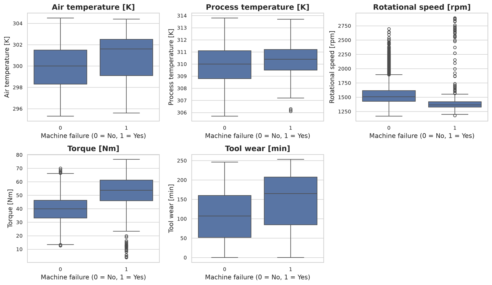
To see the shape of the risk, we split each reading into five equal sized groups and measured the failure rate in each.
Table 3: Failure rate by fifth of each reading, from lowest to highest values
| Reading | Lowest | 2nd | 3rd | 4th | Highest |
|---|---|---|---|---|---|
| Air temp | 2.1% | 2.5% | 2.0% | 3.2% | 7.2% |
| Process temp | 2.5% | 1.7% | 4.8% | 4.3% | 3.9% |
| Speed | 12.2% | 1.4% | 0.6% | 0.5% | 2.3% |
| Torque | 2.4% | 0.5% | 0.6% | 2.2% | 11.5% |
| Tool wear | 2.4% | 2.1% | 2.3% | 2.1% | 8.1% |
The risk is not a straight line. Speed and torque are U shaped, safest in the middle and riskiest at one extreme, and tool wear is flat until the last fifth, where it jumps to 8.1%.
3. Hypotheses
The exploration gave us five claims to test with models:
- H1Torque and rotational speed are the strongest signals, since their distributions separate the most.
- H2The relationship between readings and failure is non linear, so linear models will struggle and models that learn thresholds will do better.
- H3Tool wear matters, but mostly at its extreme.
- H4Temperature is weak on its own but may still help in combination with other readings.
- H5Machines slow down as they wear, which would explain why failed runs have lower average speed.
We flagged H5 early as one we could not settle here: it is about a single machine changing over time, and this dataset has no machine histories.
4. Methods
Each model was chosen to answer a question, not to try everything in a library:
Table 4: Candidate models and why each one is in the comparison
| Model | Why we chose it | Question it answers |
|---|---|---|
| Logistic regression | Simple, fast, one weight per feature | Is a straight line boundary enough? |
| Balanced logistic regression | Missed failures weigh about 28 times more | Does reweighting fix the imbalance? |
| SVM, RBF kernel | Kernel trick bends the boundary | Does a smooth curved boundary help? |
| Random Forest, 200 trees | Trees learn threshold rules | Do threshold rules match the risk shape? |
| Balanced Random Forest | Same forest with class weights | Does reweighting help the forest too? |
- Logistic regression is the baseline. If H2 is right, its single straight boundary cannot follow U shaped risk.
- The SVM uses the kernel trick: an RBF kernel compares runs by similarity, which lets it draw a curved boundary without us building features by hand. We wrapped it in sigmoid calibration so it outputs probabilities like the other models.
- Random Forests split on thresholds such as torque above a value, which is exactly the shape Table 3 shows. Averaging 200 trees reduces the variance of a single tree, and the forest reports which features it relies on, which lets us check H1, H3, and H4.
All models share one pipeline: numeric readings are standardized and the product type is one hot encoded, fitted inside each training fold so no statistics leak from validation data. The data is split 80/20 with stratification, giving 8,000 training and 2,000 test runs with the same 3.4% failure rate. Models are compared by 5 fold stratified cross validation on the training set, using the F1 score of the failure class as the main metric, because it rewards catching failures (recall) and keeping alerts trustworthy (precision) at the same time. The test set is used last.
5. Results
Table 5a: 5 fold cross validation on the training set, failure class
| Model | Precision | Recall | F1 | F1 std |
|---|---|---|---|---|
| Balanced Random Forest | 0.718 | 0.660 | 0.688 | 0.034 |
| Random Forest | 0.938 | 0.543 | 0.682 | 0.074 |
| SVM, RBF kernel | 0.297 | 0.886 | 0.445 | 0.013 |
| Logistic regression | 0.738 | 0.177 | 0.281 | 0.044 |
| Balanced logistic regression | 0.141 | 0.820 | 0.241 | 0.006 |
Both forests clearly lead. The balanced forest wins on F1 and is about twice as stable across folds as the unweighted one (0.034 against 0.074), so it became our candidate.
Table 5b: Held out test set at the default threshold of 0.5
| Model | Accuracy | Precision | Recall | F1 |
|---|---|---|---|---|
| Logistic regression | 0.971 | 0.727 | 0.235 | 0.356 |
| Balanced logistic regression | 0.808 | 0.122 | 0.750 | 0.210 |
| SVM, RBF kernel | 0.975 | 0.774 | 0.353 | 0.485 |
| Balanced Random Forest | 0.976 | 0.679 | 0.559 | 0.613 |
| Random Forest | 0.979 | 0.783 | 0.529 | 0.632 |
Accuracy hardly moves between models while F1 nearly doubles, which is why accuracy alone would have told us nothing. The unweighted forest edges ahead on this single split; we kept the cross validated choice, which averages five splits instead of one.
The SVM did better than logistic regression but never balanced the two sides: in cross validation it caught 89% of failures with only 30% of its alerts real, and on the test set it swung the other way, catching 35%. Reweighting logistic regression showed the same problem in its purest form: recall jumped from 24% to 75% while precision collapsed from 73% to 12%.
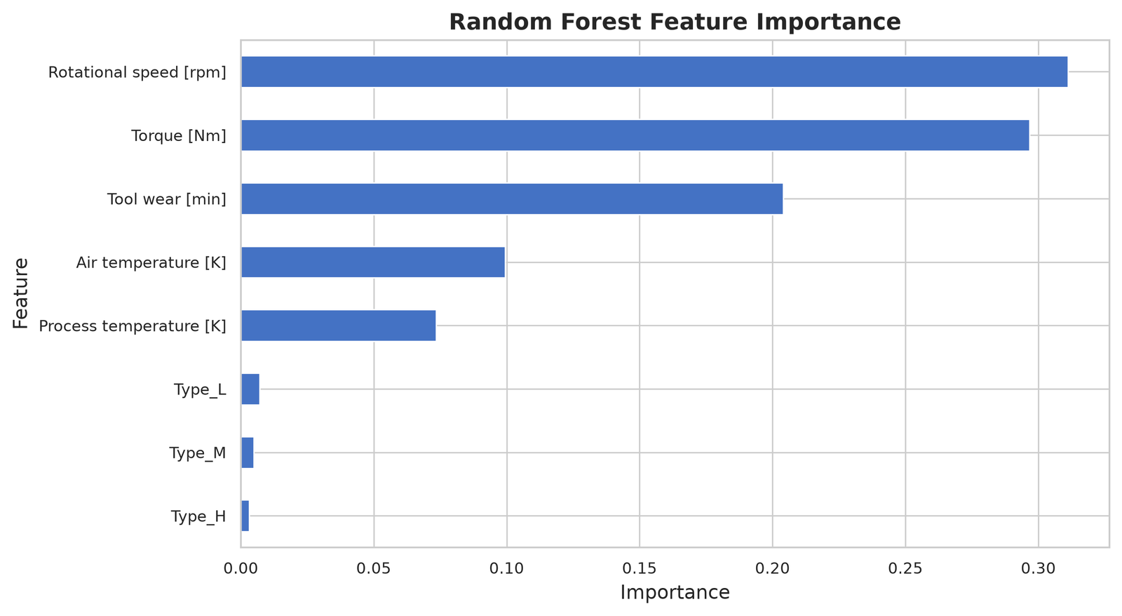
Table 6: The hypotheses against the evidence
| Hypothesis | Evidence | Verdict |
|---|---|---|
| H1 Torque and speed lead | Top two features, 61% of importance | Supported |
| H2 Non linear risk | Forest F1 0.688 against 0.281 for the linear baseline | Supported |
| H3 Tool wear at the extreme | Third feature, 0.204; but see the error analysis | Partly |
| H4 Temperature helps a little | Together about 17% of importance | Supported |
| H5 Machines slow down | Needs machine histories over time | Open |
Feature importance describes how the trained forest makes its predictions. It does not prove that raising torque causes failure, and correlated readings such as torque and speed can share importance between them.
6. Choosing a Threshold Without Peeking
A forest outputs a probability, and the threshold that turns it into an alert is a decision in its own right. Our first attempt picked the threshold that maximized F1 on the test set: 0.40, with an F1 of 0.639. We then caught the flaw. Choosing anything with the test labels makes the test score optimistic, because the test set is no longer unseen.
The corrected procedure uses the training set only. We produced out of fold probabilities with 5 fold cross validation, so every training run is scored by a model that never saw it, picked the threshold with the best F1 there (0.52, cross validated F1 0.697), refit the forest on all training data, and applied 0.52 once to the test set.
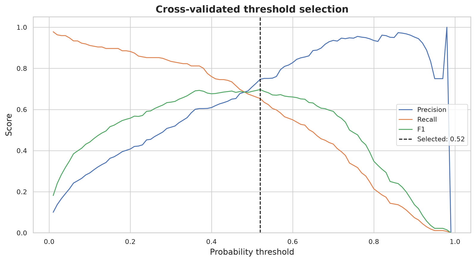
Table 7: Operating points the plant could choose (cross validated, training set)
| Threshold | Precision | Recall | F1 |
|---|---|---|---|
| 0.20 | 0.408 | 0.882 | 0.558 |
| 0.30 | 0.514 | 0.834 | 0.636 |
| 0.40 | 0.609 | 0.760 | 0.677 |
| 0.52 | 0.747 | 0.653 | 0.697 |
| 0.60 | 0.828 | 0.550 | 0.661 |
| 0.70 | 0.936 | 0.432 | 0.591 |
At 0.30 the model would catch about 83% of failures with half of its alerts real; at 0.70 almost every alert is real but fewer than half of failures are caught.
Baseline: logistic regression
Final: balanced forest at 0.52
The honest result on the test set is precision 0.69, recall 0.53, and F1 0.60. It is lower than the 0.639 from the first attempt, and it is the number we report. Compared with the baseline, the final model catches more than twice as many failures (36 against 16) for 10 extra false alarms.
7. Error Analysis
The final model still misses 32 of 68 failures. To understand why, we compared the failures it caught with the ones it missed.
Table 8: Median readings of caught and missed failures on the test set
| Reading | Caught (36) | Missed (32) |
|---|---|---|
| Torque (Nm) | 55.40 | 47.65 |
| Rotational speed (rpm) | 1,356 | 1,440 |
| Tool wear (min) | 120.5 | 165.0 |
| Air temperature (K) | 301.90 | 300.65 |
| Process temperature (K) | 310.55 | 310.70 |
| Model's failure probability | 0.74 | 0.22 |
- It learned the main pattern well. Caught failures sit at high torque and low speed, the dominant failure zone in Table 3. Failures at moderate torque look normal to the model.
- Wear related failures slip through. Missed failures had more tool wear (median 165 minutes against 120.5), so the model leans on torque and speed and underweights wear when the other readings look ordinary.
- The other end of the U is rare. Two missed failures ran at about 2,500 to 2,700 rpm with only 11 to 13 Nm of torque. High speed, low torque failures are uncommon in the training data, so the forest has few examples to learn them from.
- Some misses cannot be fixed by the threshold. A quarter of the missed failures received a probability of 0.06 or less, the lowest close to 0. No threshold catches those; they need new information, not a different cut off.
8. Limitations
- The data is a synthetic benchmark and may not match a particular factory, machine fleet, or maintenance policy.
- A random split can be optimistic when runs depend on each other over time.
- F1 weighs precision and recall equally; a real plant should weigh them by cost.
- The forest's probabilities are not calibrated, so 0.7 does not yet mean a 70% chance of failure.
9. What We Recommend Next
- Engineer physical features. The dataset documentation defines three failure modes with combined quantities: power (torque times angular speed) outside 3,500 to 9,000 W, overstrain when tool wear times torque passes 11,000 to 13,000 min·Nm depending on product type, and heat dissipation when the gap between process and air temperature is under 8.6 K at speeds under 1,380 rpm. The failure flags in the data follow these rules exactly. A forest has to approximate a product like torque times speed with many single feature splits, so giving it power, strain, and the temperature gap directly should help most with the missed high speed, low torque and high wear cases.
- Set the threshold from costs. Price a missed failure and an unnecessary inspection, account for how many alerts the crew can handle, and pick the operating point in Table 7 that minimizes total cost instead of maximizing F1.
- Try gradient boosting. It was on our original plan and is the natural next comparison, since it builds trees one after another to fix the previous trees' mistakes, including the rare failure patterns.
- Calibrate, then validate on real time ordered data. Calibrated probabilities would let a planner read the score as a real risk. Validating on machine histories ordered in time would give an honest estimate for deployment and is the only way to test H5.
Reproducibility
The analysis started in two Jupyter notebooks, one for exploration and one for modeling, and was then refactored into a small Python package so the notebooks and the training script share the same code. A single command retrains all five candidates, selects the threshold with cross validation, and saves the production pipeline, the threshold, the metrics, and every figure on this page.
A solo personal project: I did the analysis, the modeling, and the pipeline end to end.
References
- [1]Siemens, Senseye Predictive Maintenance. The True Cost of Downtime 2024. assets.new.siemens.com
- [2]U.S. Department of Energy, Federal Energy Management Program. Operations & Maintenance Best Practices: A Guide to Achieving Operational Efficiency, Release 2.0 (PNNL 14788), 2004, section 5.4. pnnl.gov
- [3]UCI Machine Learning Repository. AI4I 2020 Predictive Maintenance Dataset. archive.ics.uci.edu
 Python
 scikit-learn
 Pandas
 NumPy